Often you may want to highlight an entire row in Excel based on a given cell value in the row.
For example, you may want to highlight each row in the following dataset in which the value in the Passed column is “Yes”:
This is easy to do using the Conditional Formatting feature in Excel.
The following example shows how to do so in practice.
Example: Highlight Entire Row Based on Cell Value in Excel
Suppose we have the following dataset in Excel that contains information on the total hours studied, final exam score, and passing status of various students in some class:
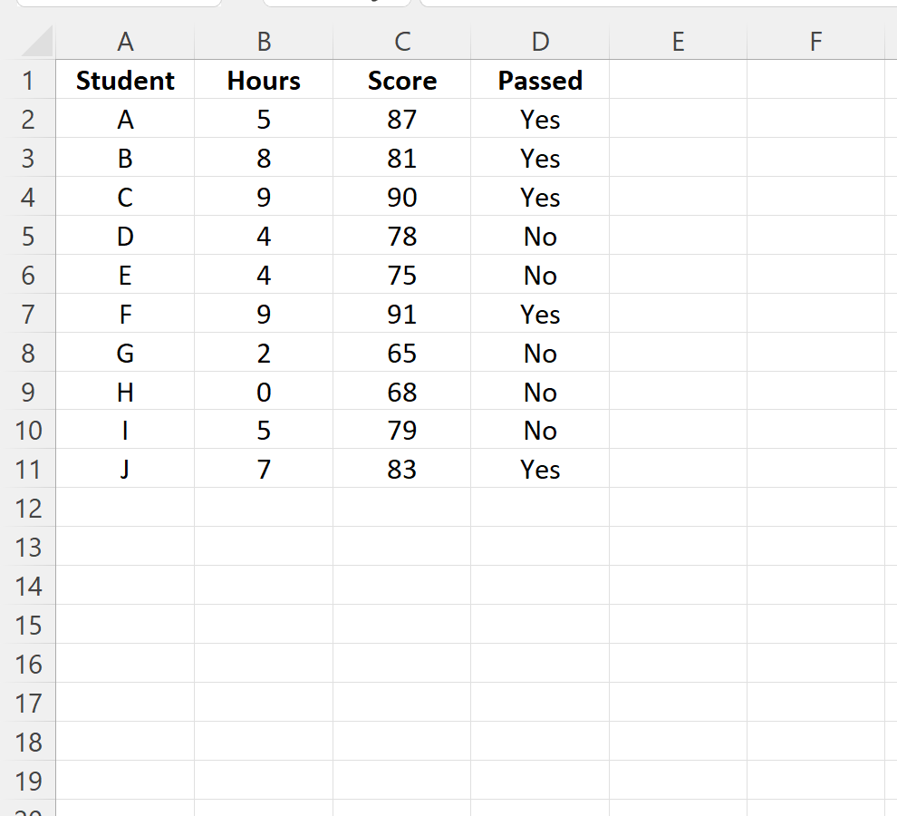
Now suppose that we would like to highlight each row in which the value in the Passed column is “Yes.”
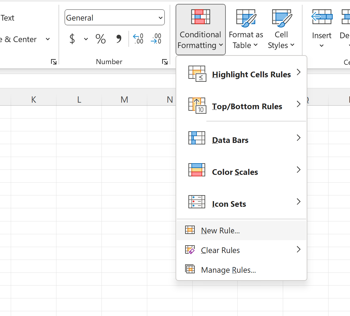
To do so, we can highlight the cell range A2:D11, then click the Conditional Formatting icon, then click New Rule:
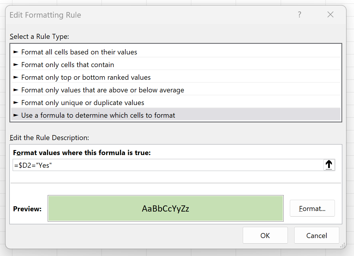
In the new window that appears, click the option called Use a formula to determine which cells to format, then type =$D2=”Yes” in the box, then click the Format button and choose a fill color to use:
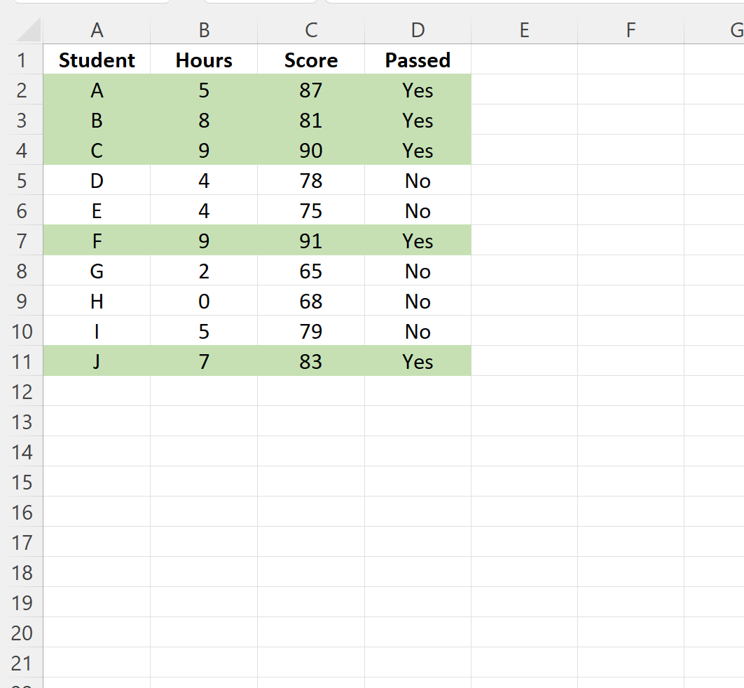
Once you click OK, each of the rows that contain a “Yes” in the Passed column will be highlighted:
Each row that contains “Yes” in the Passed column now has a fill color of light green while each row that contains “No” is left unchanged.
Note that for this example we chose to highlight the rows using a light green, but you can choose any color you’d like by selecting a different color using the Format button within the Edit Formatting Rule window.
Additional Resources
The following tutorials explain how to perform other common tasks in Excel:
How to Filter by List of Values in Excel
How to Filter a Column by Multiple Values in Excel
How to Count Rows with Value in Excel