You can use the following basic formula to perform a VLOOKUP with two lookup values in Excel:
=VLOOKUP(F1&F2,CHOOSE({1,2},A2:A10&B2:B10,C2:C10),2,FALSE)
This particular formula looks up the values in F1 and F2 in the ranges A2:A10 and B2:B10, respectively, and returns the corresponding value in the range C2:C10.
The following example shows how to use this formula in practice.
Example: Perform VLOOKUP with Two Lookup Values
Suppose we have the following dataset in Excel that shows the points scored by various basketball players:

Now suppose we would like to use a VLOOKUP function to find the points value that corresponds to a Team value of Mavs and a Position value of Center.
To do so, we can type the following formula into cell F3:
=VLOOKUP(F1&F2,CHOOSE({1,2},A2:A10&B2:B10,C2:C10),2,FALSE)
The following screenshot shows how to use this formula in practice:
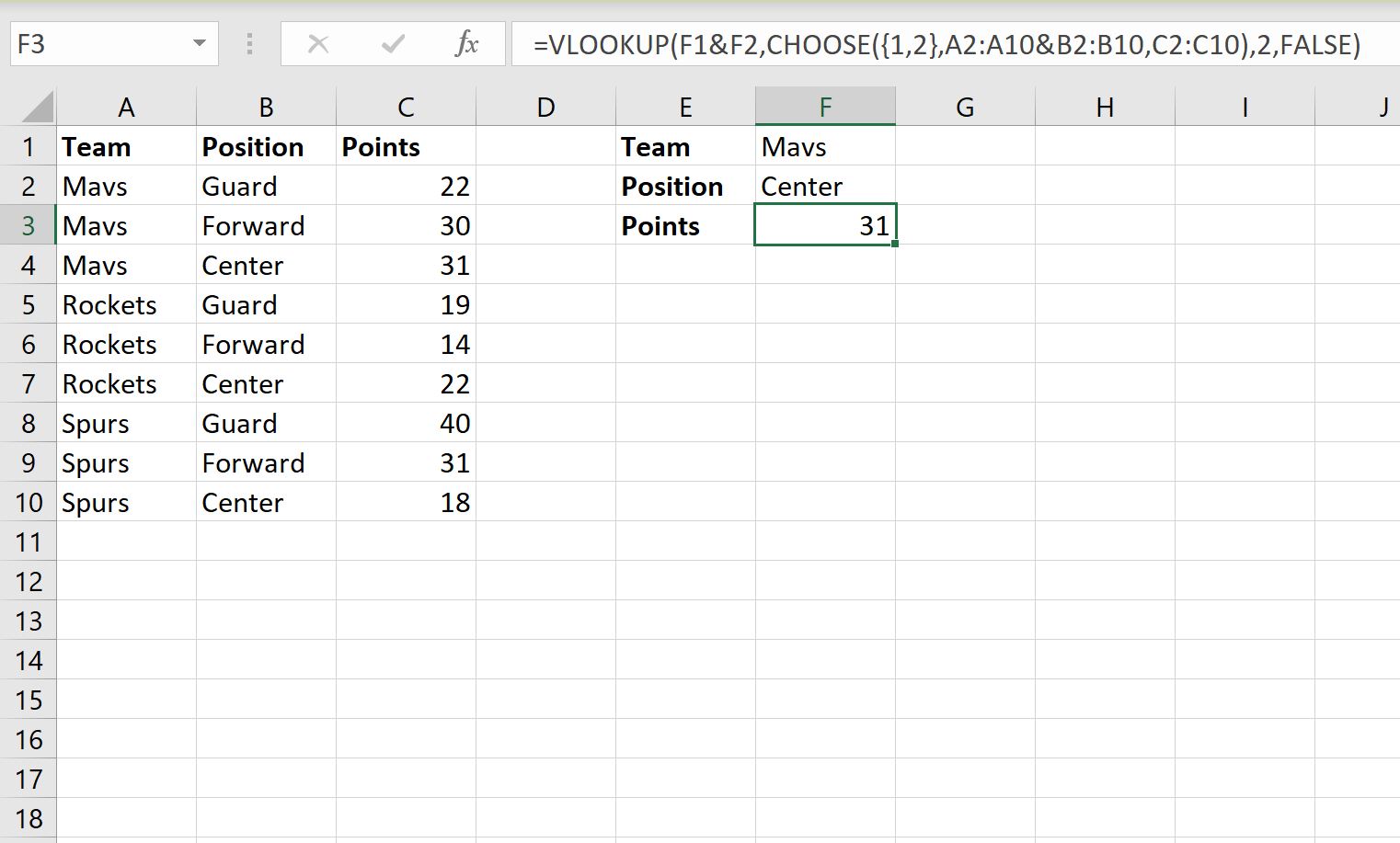
The formula returns a value of 31.
This is the correct points value that corresponds to the player on the Mavs team who has a position of Center.
Note that we can change the values in column F to find the points value for a different player.
For example, if we change the Team to Spurs and the Position to Guard, the VLOOKUP function will automatically update to find the points value for this player:
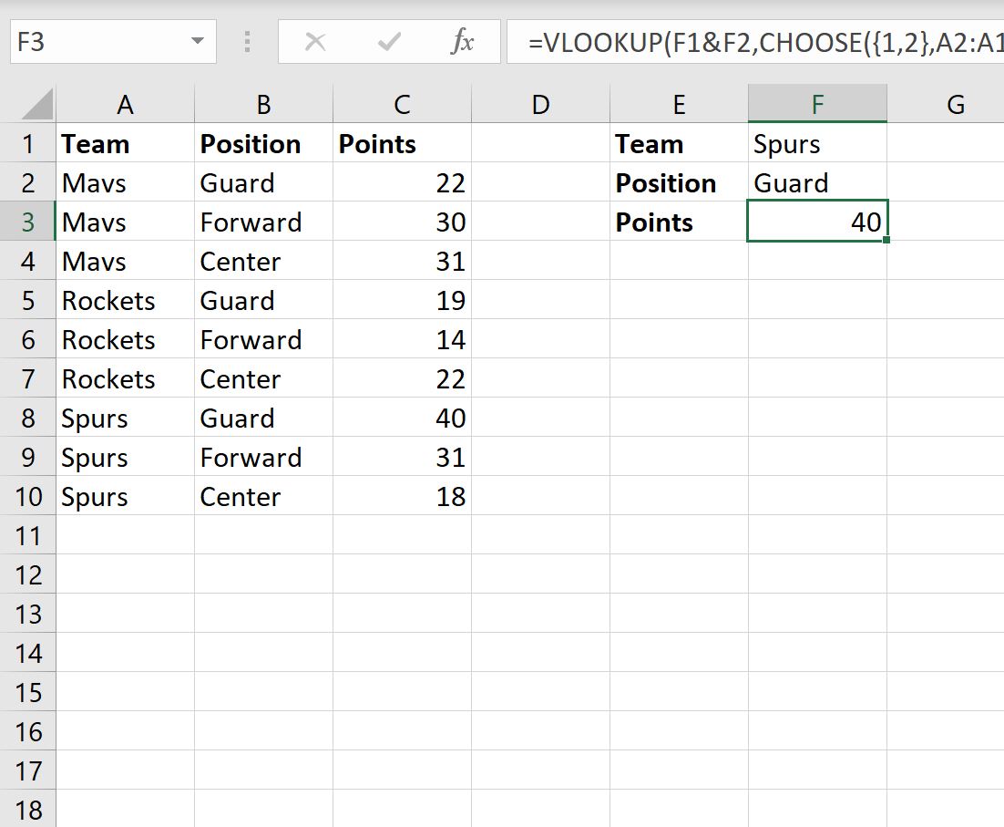
The formula returns the correct points value of 40.
Additional Resources
The following tutorials explain how to perform other common tasks in Excel:
How to Calculate a Weighted Percentage in Excel
How to Multiply Column by a Percentage in Excel
How to Calculate Percentile Rank in Excel