Occasionally you may want to add a vertical line to a chart in Excel at a specific position.
This tutorial provides a step-by-step example of how to add a vertical line to the following line chart in Excel:

Let’s jump in!
Step 1: Enter the Data
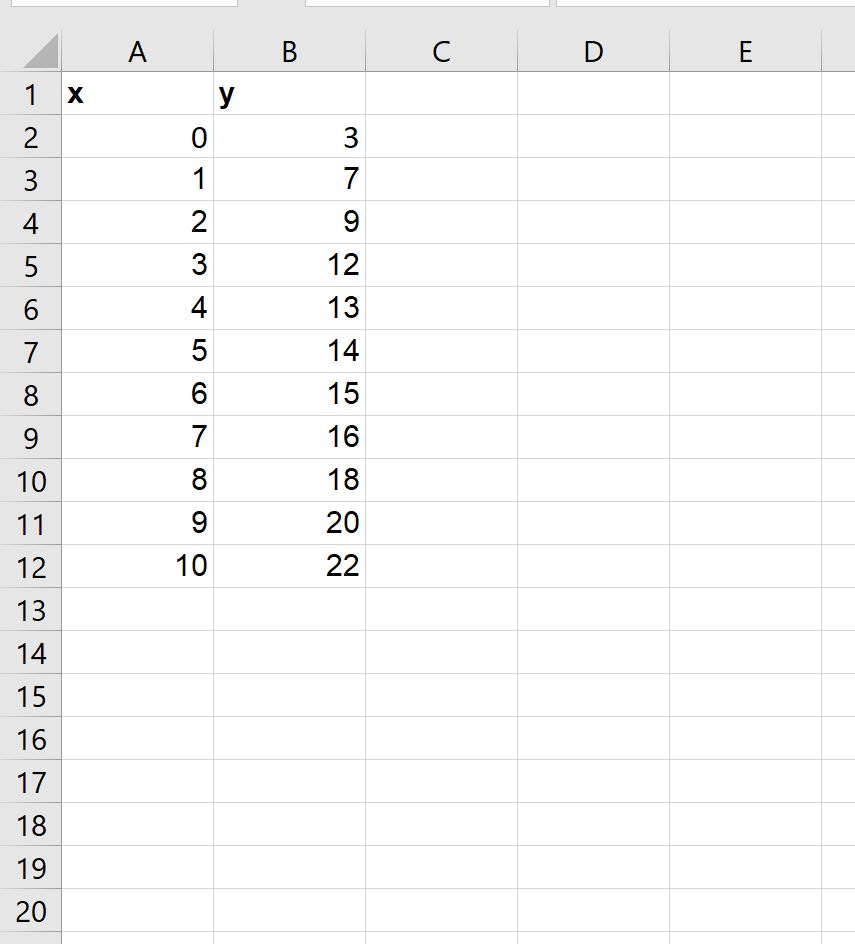
Suppose we would like to create a line chart using the following dataset in Excel:
Step 2: Add Data for Vertical Line
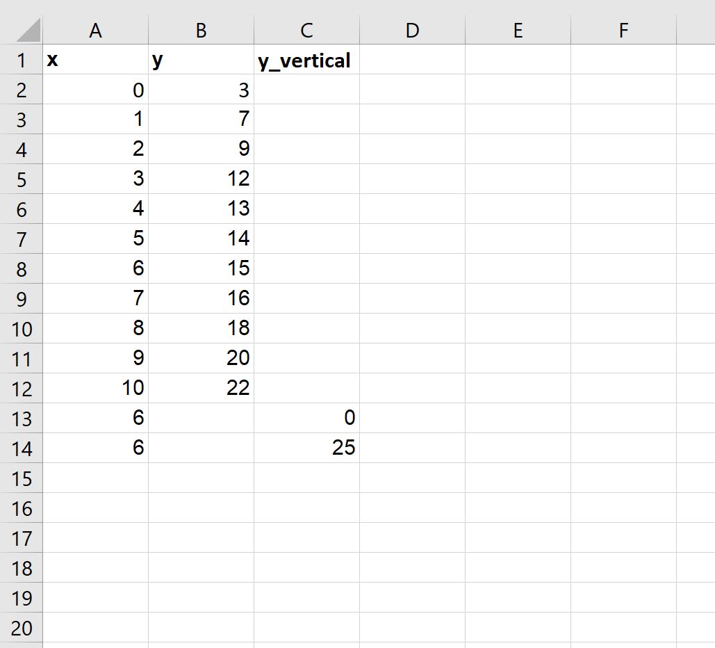
Now suppose we would like to add a vertical line located at x = 6 on the plot.
We can add in the following artificial (x, y) coordinates to the dataset:
Step 3: Create Line Chart with Vertical Line
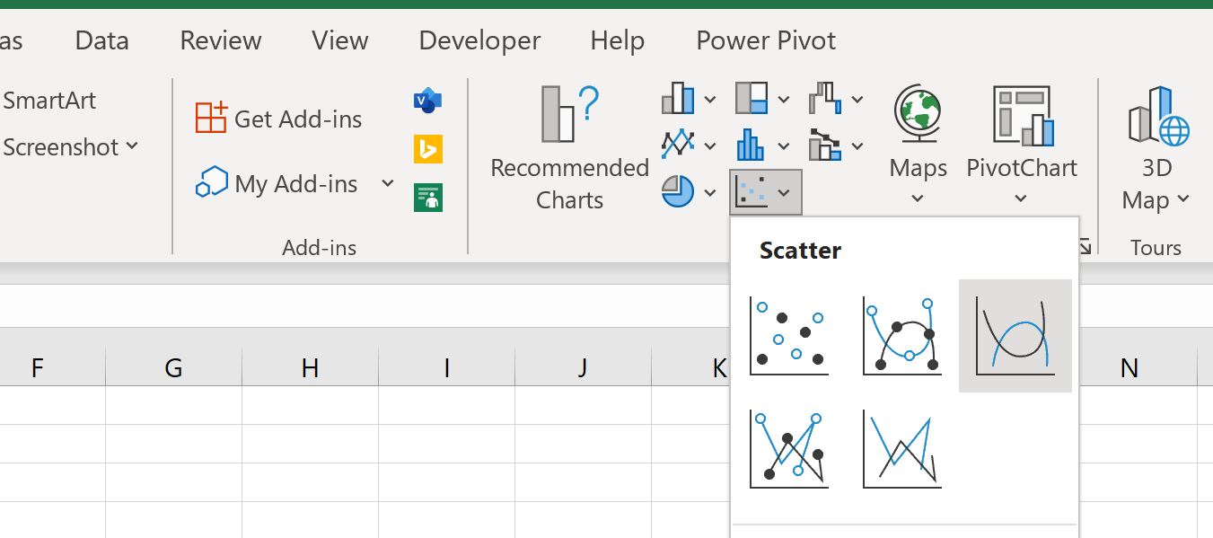
Lastly, we can highlight the cells in the range A2:C14, then click the Insert tab along the top ribbon, then click Scatter with Smooth Lines within the Charts group:
The following line chart will be created:
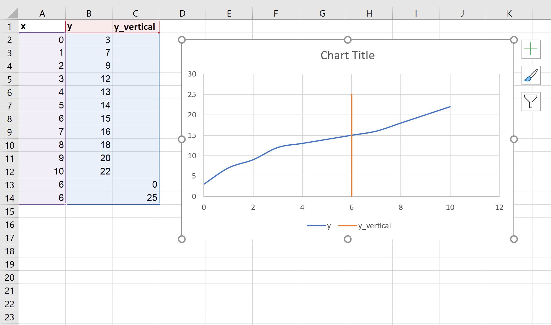
Notice that the vertical line is located at x = 6, which we specified at the end of our original dataset.
The vertical line ranges from y = 0 to y =25, which we also specified in our original dataset.
To change the height of the line, simply change the y-values to use whatever starting and ending points you’d like.
Step 4: Customize the Chart (Optional)
Lastly, feel free to modify the range of each axis along with the style of the vertical line to make it more aesthetically pleasing:
Additional Resources
The following tutorials explain how to perform other common tasks in Excel:
How to Add Average Line to Bar Chart in Excel
How to Add a Horizontal Line to Scatterplot in Excel