Occasionally you may want to add a horizontal line to a scatterplot in Excel to represent some threshold or limit.
This tutorial provides a step-by-step example of how to quickly add a horizontal line to any scatterplot in Excel.
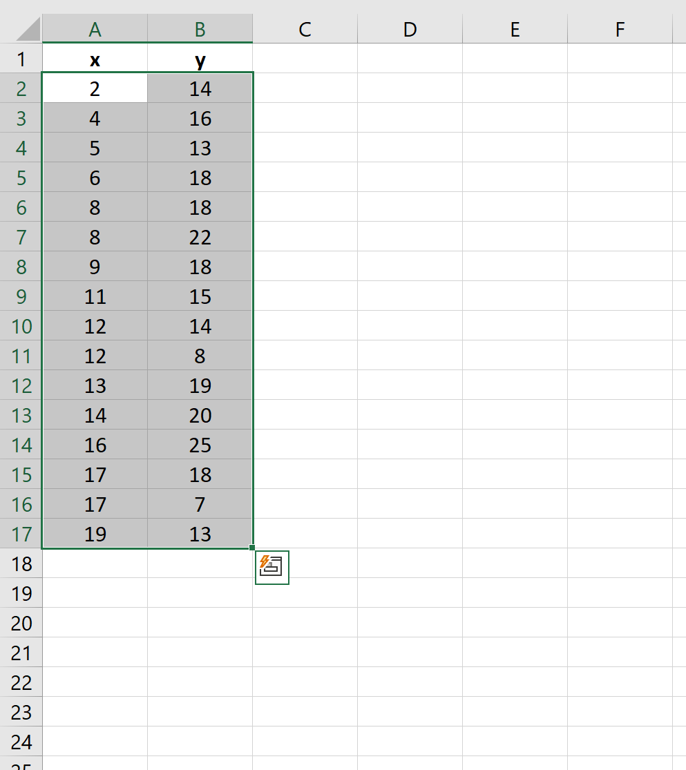
Step 1: Create the Data
First, let’s create the following fake dataset:

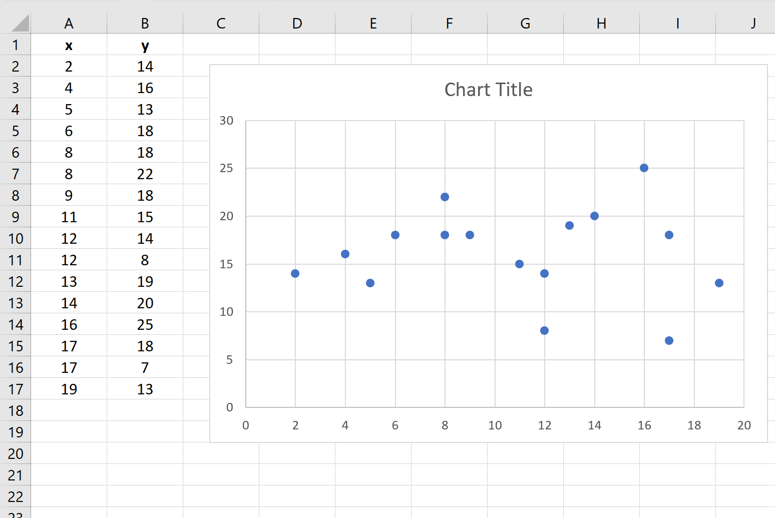
Step 2: Create the Scatterplot
Next, highlight the data in the cell range A2:B17 as follows:
Along the top ribbon, click Insert and then click the first chart in the Insert Scatter (X, Y) or Bubble Chart group within the Charts group. The following scatterplot will automatically appear:
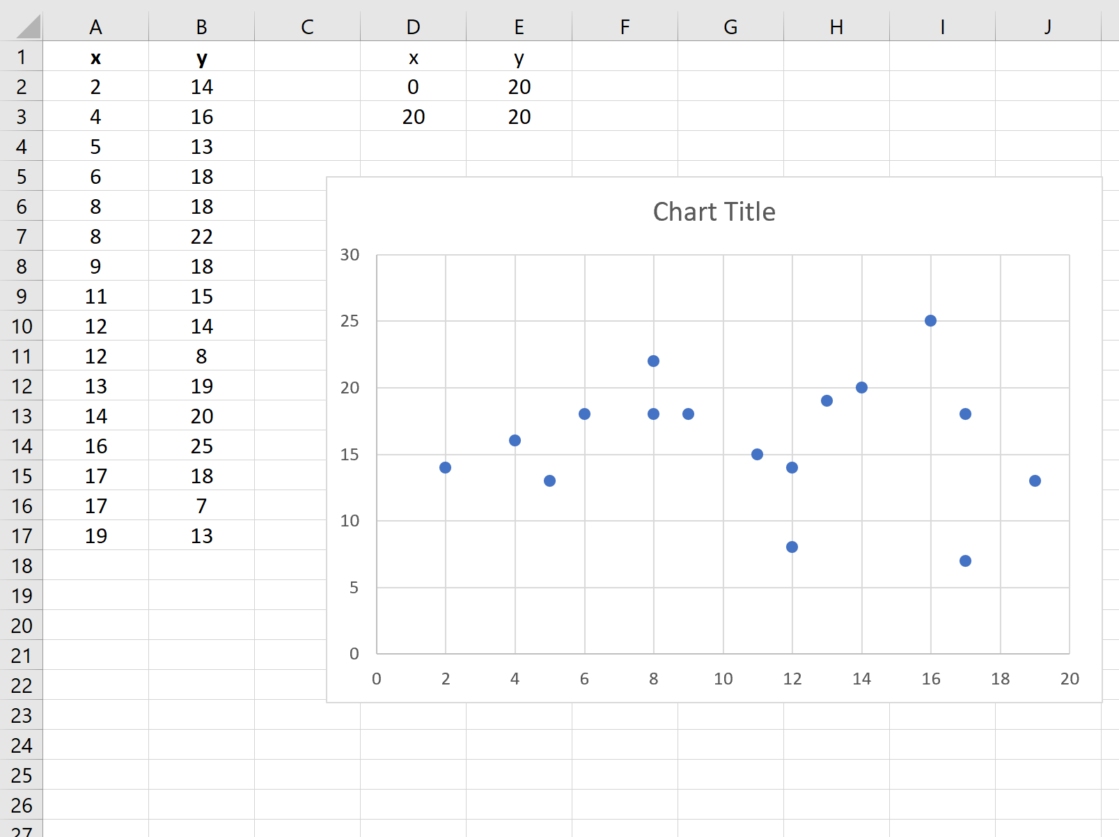
Step 3: Add a Horizontal Line
Now suppose we would like to add a horizontal line at y = 20.
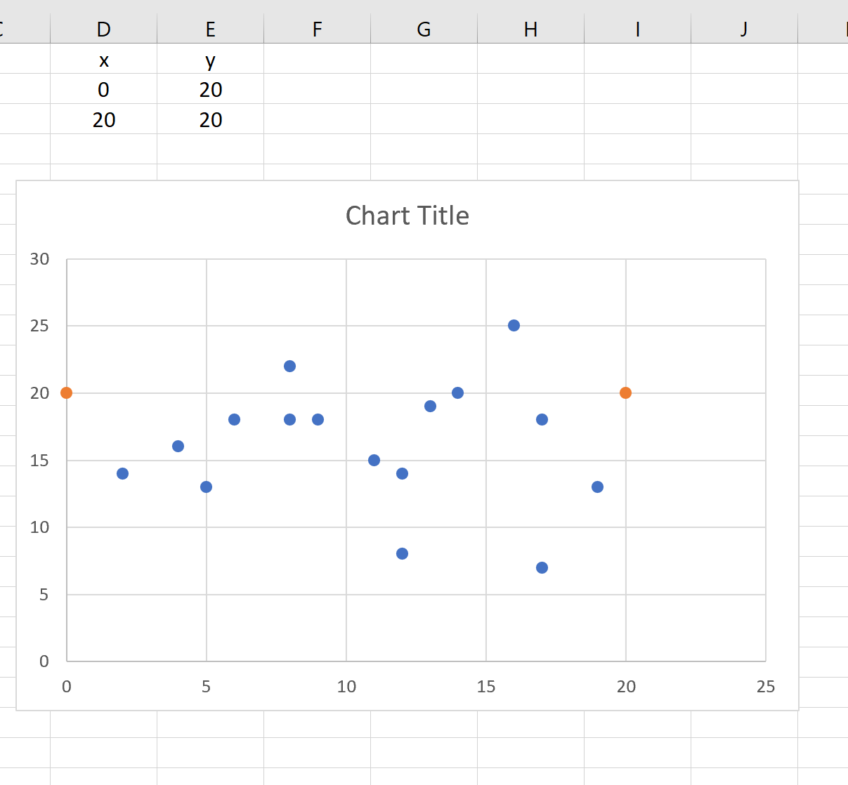
To do this, we can create a fake data series that shows the minimum and maximum value along the x-axis (0 and 20) as well as two y-values that are both equal to 20:
Next, right click anywhere on the chart and click Select Data. In the window that appears, click Add under the Legend Entries (Series) section.
In the new window that appears, fill in the following information:
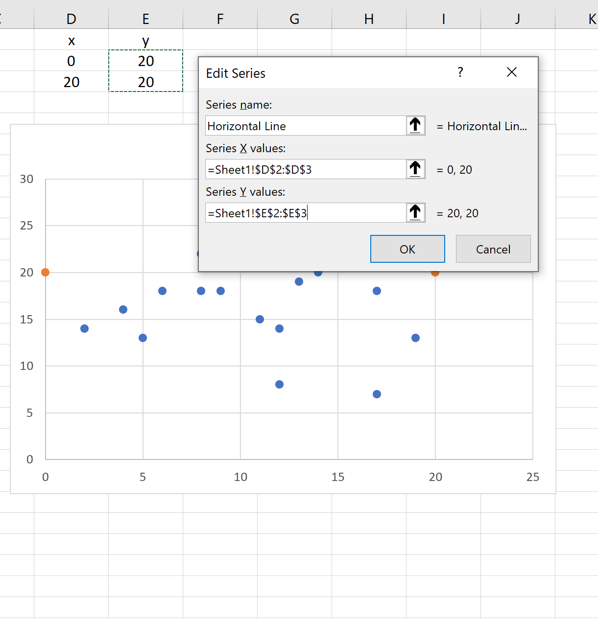
Once you click OK, two orange dots will appear on the chart:
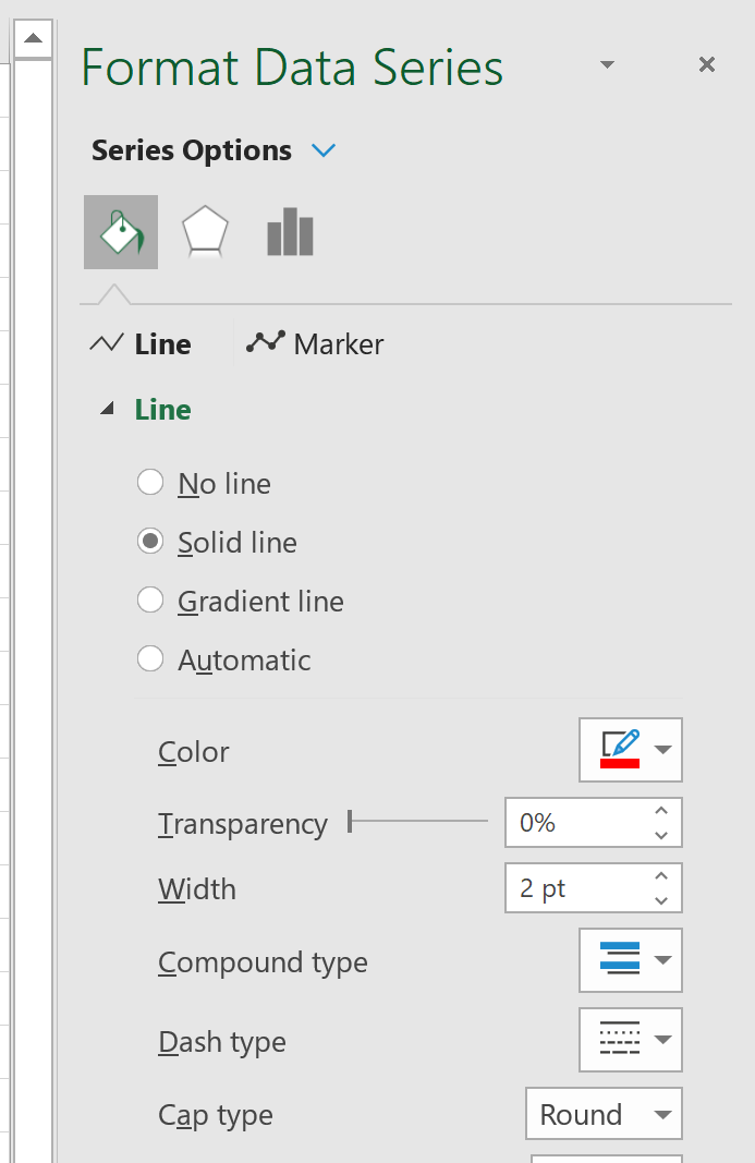
Right click on one of the orange dots and click Format Data Series…
In the window that appears on the right side of the screen, click Solid Line:
This will turn the two orange points into a solid orange line:
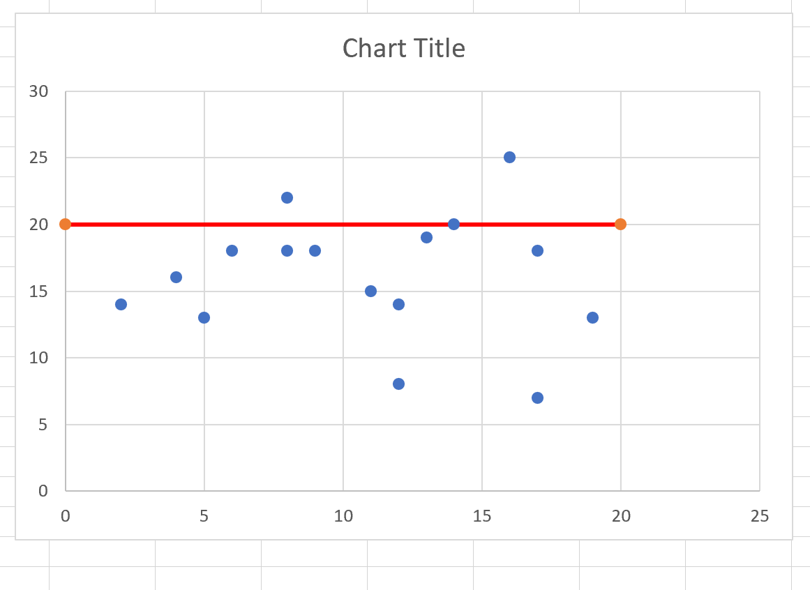
Feel free to modify the color, thickness, and style of the line to make it more aesthetically pleasing.
If you would like to add multiple horizontal lines to a single chart, simply repeat this process using different y-values.
Related: How to Add Average Line to Bar Chart in Excel
Additional Resources
The following tutorials explain how to perform other common tasks in Excel:
How to Fit a Curve in Excel
How to Make a Frequency Polygon in Excel
How to Create a Bland-Altman Plot in Excel