How to Match Two Columns and Return a Third in Excel

by Tutor Aspire February 17, 2016

Often you may want to match the values in two columns and output a third column in Excel.

Fortunately this is easy to do using the VLOOKUP() function, which uses the following syntax:

VLOOKUP(lookup_value, table_array, col_index_num, [range_lookup])

where:

lookup_value: The value you want to look up.
table_array: The range of cells to look in.
col_index_num: The column number in the range that contains the return value.
range_lookup: Whether to find an approximate match (default) or exact match.

The following example shows how to use this function to match two columns and return a third in Excel.

Suppose we have the following datasets in Excel:

Suppose we would like to match the team values in column A and column D and return the points values in column B into column E.

We can use the following VLOOKUP syntax to match the first value in column A:

=VLOOKUP(D2, $A$2:$B$16, 2, FALSE)

The following screenshot shows how to use this syntax in practice:

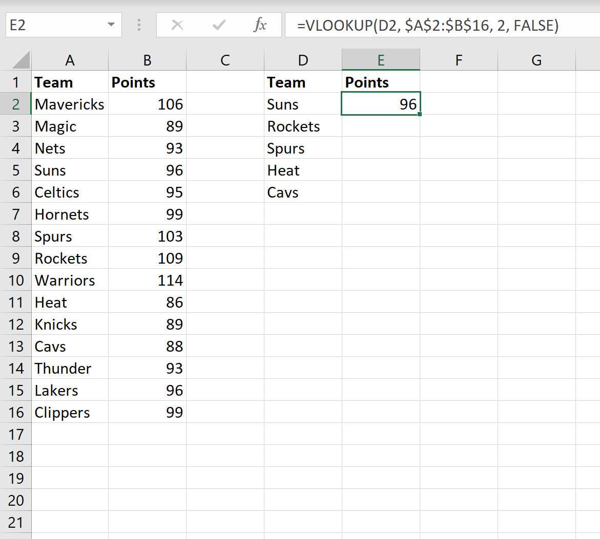
Notice that the ‘points’ value in column B that corresponds to ‘Suns’ is 96, which is why this value is returned in column E.

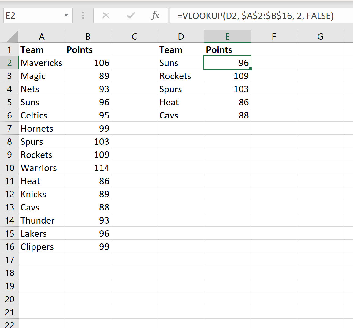
We can then drag this formula down to every remaining cell in column E:

Note: You can find the complete documentation for the VLOOKUP function here.

The following tutorials explain how to perform other common operations in Excel: