Exponential regression is a type of regression that can be used to model the following situations:
1. Exponential growth: Growth begins slowly and then accelerates rapidly without bound.

2. Exponential decay: Decay begins rapidly and then slows down to get closer and closer to zero.

The equation of an exponential regression model takes the following form:
y = abx
where:
- y: The response variable
- x: The predictor variable
- a, b: The regression coefficients that describe the relationship between x and y
The following step-by-step example shows how to perform exponential regression in R.
Step 1: Create the Data
First, let’s create some fake data for two variables: x and y:
x=1:20
y=c(1, 3, 5, 7, 9, 12, 15, 19, 23, 28, 33, 38, 44, 50, 56, 64, 73, 84, 97, 113)
Step 2: Visualize the Data
Next, let’s create a quick scatterplot to visualize the relationship between x and y:
plot(x, y)
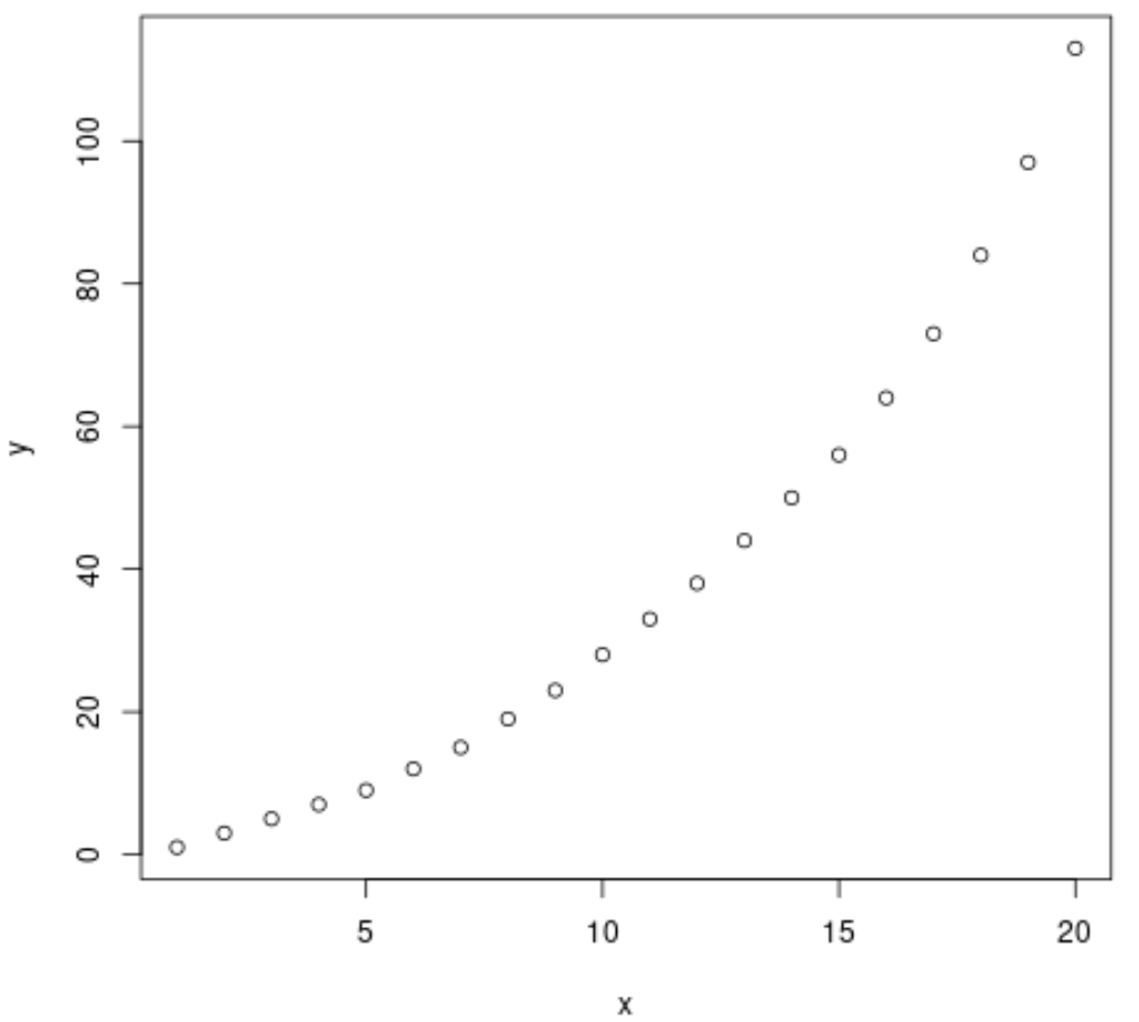
From the plot we can see that there exists a clear exponential growth pattern between the two variables.
Thus, it seems like a good idea to fit an exponential regression equation to describe the relationship between the variables.
Step 3: Fit the Exponential Regression Model
Next, we’ll use the lm() function to fit an exponential regression model, using the natural log of y as the response variable and x as the predictor variable:
#fit the model
model log(y)~ x)

#view the output of the model
summary(model)

Call:
lm(formula = log(y) ~ x)

Residuals:
    Min      1Q  Median      3Q     Max
-1.1858 -0.1768  0.1104  0.2720  0.3300

Coefficients:
            Estimate Std. Error t value Pr(>|t|)
(Intercept)  0.98166    0.17118   5.735 1.95e-05 ***
x            0.20410    0.01429  14.283 2.92e-11 ***
---
Signif. codes:  0 ‘***’ 0.001 ‘**’ 0.01 ‘*’ 0.05 ‘.’ 0.1 ‘ ’ 1

Residual standard error: 0.3685 on 18 degrees of freedom
Multiple R-squared:  0.9189,	Adjusted R-squared:  0.9144
F-statistic:   204 on 1 and 18 DF,  p-value: 2.917e-11
The overall F-value of the model is 204 and the corresponding p-value is extremely small (2.917e-11), which indicates that the model as a whole is useful.
Using the coefficients from the output table, we can see that the fitted exponential regression equation is:
ln(y) = 0.9817 + 0.2041(x)
Applying e to both sides, we can rewrite the equation as:
y = 2.6689 * 1.2264x
We can use this equation to predict the response variable, y, based on the value of the predictor variable, x. For example, if x = 12, then we would predict that y would be 30.897:
y = 2.6689 * 1.226412 = 30.897
Bonus: Feel free to use this online Exponential Regression Calculator to automatically compute the exponential regression equation for a given predictor and response variable.
Additional Resources
How to Perform Simple Linear Regression in R
How to Perform Multiple Linear Regression in R
How to Perform Quadratic Regression in R
How to Perform Polynomial Regression in R