How to Perform Multiple Linear Regression in R

This guide walks through an example of how to conduct multiple linear regression in R, including:

Examining the data before fitting the model
Fitting the model
Checking the assumptions of the model
Interpreting the output of the model
Assessing the goodness of fit of the model
Using the model to make predictions

Let’s jump in!

Setup

For this example we will use the built-in R dataset mtcars, which contains information about various attributes for 32 different cars:

#view first six lines of mtcars
head(mtcars)

#                   mpg cyl disp  hp drat    wt  qsec vs am gear carb
#Mazda RX4         21.0   6  160 110 3.90 2.620 16.46  0  1    4    4
#Mazda RX4 Wag     21.0   6  160 110 3.90 2.875 17.02  0  1    4    4
#Datsun 710        22.8   4  108  93 3.85 2.320 18.61  1  1    4    1
#Hornet 4 Drive    21.4   6  258 110 3.08 3.215 19.44  1  0    3    1
#Hornet Sportabout 18.7   8  360 175 3.15 3.440 17.02  0  0    3    2
#Valiant           18.1   6  225 105 2.76 3.460 20.22  1  0    3    1

In this example we will build a multiple linear regression model that uses mpg as the response variable and disp, hp, and drat as the predictor variables.

#create new data frame that contains only the variables we would like to use to
data #view first six rows of new data frame
head(data)

#                   mpg disp  hp drat
#Mazda RX4         21.0  160 110 3.90
#Mazda RX4 Wag     21.0  160 110 3.90
#Datsun 710        22.8  108  93 3.85
#Hornet 4 Drive    21.4  258 110 3.08
#Hornet Sportabout 18.7  360 175 3.15
#Valiant           18.1  225 105 2.76

Examining the Data

Before we fit the model, we can examine the data to gain a better understanding of it and also visually assess whether or not multiple linear regression could be a good model to fit to this data.

In particular, we need to check if the predictor variables have a linear association with the response variable, which would indicate that a multiple linear regression model may be suitable.

To do so, we can use the pairs() function to create a scatterplot of every possible pair of variables:

pairs(data, pch = 18, col = "steelblue")

From this pairs plot we can see the following:

mpg and disp appear to have a strong negative linear correlation
mpg and hp appear to have a strong positive linear correlation
mpg and drat appear to have a modest negative linear correlation

Note that we could also use the ggpairs() function from the GGally library to create a similar plot that contains the actual linear correlation coefficients for each pair of variables:

#install and load the GGally library
install.packages("GGally")
library(GGally)

#generate the pairs plot
ggpairs(data)

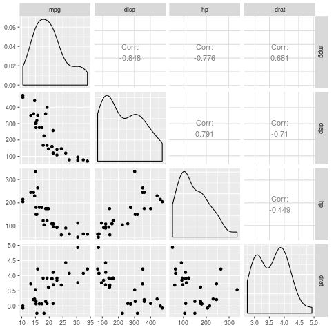
Each of the predictor variables appears to have a noticeable linear correlation with the response variable mpg, so we’ll proceed to fit the linear regression model to the data.

Fitting the Model

The basic syntax to fit a multiple linear regression model in R is as follows:

lm(response_variable ~ predictor_variable1 + predictor_variable2 + ..., data = data)

Using our data, we can fit the model using the following code:

model

Checking Assumptions of the Model

Before we proceed to check the output of the model, we need to first check that the model assumptions are met. Namely, we need to verify the following:

1. The distribution of model residuals should be approximately normal.

We can check if this assumption is met by creating a simple histogram of residuals:

hist(residuals(model), col = "steelblue")

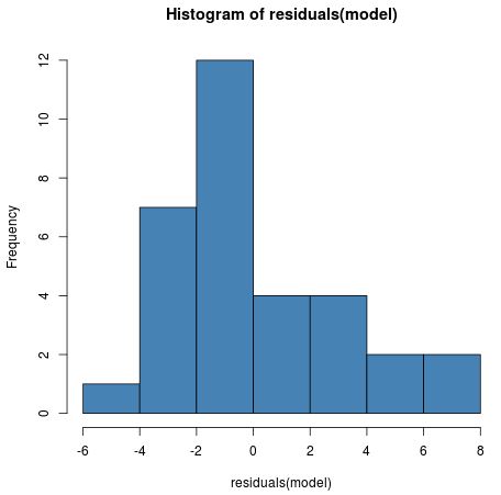
Although the distribution is slightly right skewed, it isn’t abnormal enough to cause any major concerns.

2. The variance of the residuals should be consistent for all observations.

This preferred condition is known as homoskedasticity. Violation of this assumption is known as heteroskedasticity.

To check if this assumption is met we can create a fitted value vs. residual plot:

#create fitted value vs residual plot
plot(fitted(model), residuals(model))

#add horizontal line at 0
abline(h = 0, lty = 2)

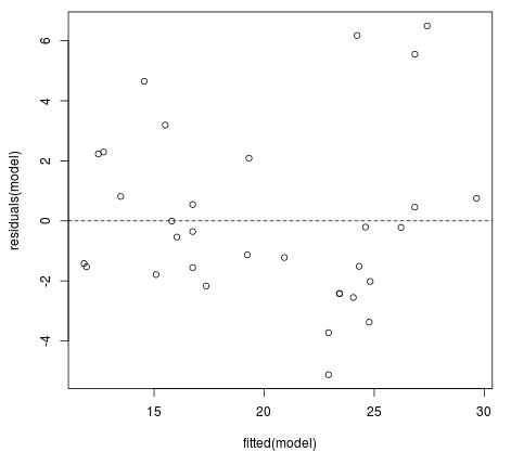
Ideally we would like the residuals to be equally scattered at every fitted value. We can see from the plot that the scatter tends to become a bit larger for larger fitted values, but this pattern isn’t extreme enough to cause too much concern.

Interpreting the Output of the Model

Once we’ve verified that the model assumptions are sufficiently met, we can look at the output of the model using the summary() function:

summary(model)

#Call:
#lm(formula = mpg ~ disp + hp + drat, data = data)
#
#Residuals:
#    Min      1Q  Median      3Q     Max 
#-5.1225 -1.8454 -0.4456  1.1342  6.4958 
#
#Coefficients:
#             Estimate Std. Error t value Pr(>|t|)   
#(Intercept) 19.344293   6.370882   3.036  0.00513 **
#disp        -0.019232   0.009371  -2.052  0.04960 * 
#hp          -0.031229   0.013345  -2.340  0.02663 * 
#drat         2.714975   1.487366   1.825  0.07863 . 
#---
#Signif. codes:  0 '***' 0.001 '**' 0.01 '*' 0.05 '.' 0.1 ' ' 1
#
#Residual standard error: 3.008 on 28 degrees of freedom
#Multiple R-squared:  0.775,	Adjusted R-squared:  0.7509 
#F-statistic: 32.15 on 3 and 28 DF,  p-value: 3.28e-09

From the output we can see the following:

The overall F-statistic of the model is 32.15 and the corresponding p-value is 3.28e-09. This indicates that the overall model is statistically significant. In other words, the regression model as a whole is useful.
disp is statistically significant at the 0.10 significance level. In particular, the coefficient from the model output tells is that a one unit increase in disp is associated with a -0.019 unit decrease, on average, in mpg, assuming hp and drat are held constant.
hp is statistically significant at the 0.10 significance level. In particular, the coefficient from the model output tells is that a one unit increase in hp is associated with a -0.031 unit decrease, on average, in mpg, assuming disp and drat are held constant.
drat is statistically significant at the 0.10 significance level. In particular, the coefficient from the model output tells is that a one unit increase in drat is associated with a 2.715 unit increase, on average, in mpg, assuming disp and hp are held constant.

Assessing the Goodness of Fit of the Model

To assess how “good” the regression model fits the data, we can look at a couple different metrics:

1. Multiple R-Squared

This measures the strength of the linear relationship between the predictor variables and the response variable. A multiple R-squared of 1 indicates a perfect linear relationship while a multiple R-squared of 0 indicates no linear relationship whatsoever.

Multiple R is also the square root of R-squared, which is the proportion of the variance in the response variable that can be explained by the predictor variables. In this example, the multiple R-squared is 0.775. Thus, the R-squared is 0.775² = 0.601. This indicates that 60.1% of the variance in mpg can be explained by the predictors in the model.

2. Residual Standard Error

This measures the average distance that the observed values fall from the regression line. In this example, the observed values fall an average of 3.008 units from the regression line.

Using the Model to Make Predictions

From the output of the model we know that the fitted multiple linear regression equation is as follows:

mpg_hat = -19.343 – 0.019*disp – 0.031*hp + 2.715*drat

We can use this equation to make predictions about what mpg will be for new observations. For example, we can find the predicted value of mpg for a car that has the following attributes:

disp = 220
hp = 150
drat = 3

#define the coefficients from the model output
intercept #use the model coefficients to predict the value for mpg
intercept + disp*220 + hp*150 + drat*3

#[1] 18.57373

For a car with disp = 220, hp = 150, and drat = 3, the model predicts that the car would have a mpg of 18.57373.

You can find the complete R code used in this tutorial here.

Additional Resources

The following tutorials explain how to fit other types of regression models in R:

How to Perform Quadratic Regression in R
How to Perform Polynomial Regression in R
How to Perform Exponential Regression in R