-
MATLAB Tutorial
- matlab-tutorial
- matlab-introduction
- platform-features
- prerequisites-system-requirements
- matlab-downloading
- matlab-installation
- matlab-online
- advantage-disadvantage
- matlab-commands
- matlab-environment
- working-with-variables-arrays
- workspace,-variables,-functions
- matlab-data-types
- matlab-operator
- formatting-text
Control Statements
- if...end-statement
- if-else...-end-statement
- if-elseif-else...end-statement
- nested-if-else
- matlab-switch
MATLAB Loops
Statement-try, catch
Program Termination
Arrays & Functions
- matlab-matrices-arrays
- multi-dimensional-arrays
- matlab-compatible-array
- matlab-sparse-matrices
- matlab-m-files
- matlab-functions
- anonymous-function
MATLAB Graphics
MATLAB 2D Plots
- matlab-fplot()
- matlab-semilogx()
- matlab-semilogy()
- matlab-loglog()
- matlab-polar-plots()
- matlab-fill()
- matlab-bar()
- matlab-errorbar()
- matlab-barh()
- matlab-plotyy()
- matlab-area()
- matlab-pie()
- matlab-hist()
- matlab-stem()
- matlab-stairs()
- matlab-compass()
- matlab-comet()
- matlab-contour()
- matlab-quiver()
- matlab-pcolor()
MATLAB 3D Plots
- matlab-3d-plots
- matlab-plot3()
- matlab-fill3()
- matlab-contour3()
- matlab-surf()
- matlab-surfc()
- matlab-mesh()
- matlab-meshz()
- matlab-waterfall()
- matlab-stem3()
- matlab-ribbon()
- matlab-sphere()
- matlab-ellipsoid()
- matlab-cylinder()
- matlab-slice()
Linear Algebra
Symbolic Mathematics
MATLAB Polynomial
Numerical Integration
- numerical-integration
- matlab-double-integral
- matlab-trapezoidal-rule
- matlab-trapz
- matlab-simpson's-rule
MATLAB GUI
MATLAB Programs
- environment-programming
- matlab-variables
- operations-on-matrices
- control-statements
- matlab-2-d-plots
- matlab-sine-wave-plot
Interview Questions
MATLAB PolynomialMATLAB performs, polynomials as row vectors, including coefficients ordered by descending powers. For example, the equation P(x) = x4 + 7x3 - 5x + 9 can be represented as - p = [1 7 0 -5 9]; Polynomial FunctionspolyfitGiven two vector x and y, the command a=polyfit (x, y, n) fits a polynomial of order n through the data points (xi,yi) and returns (n+1) coefficients of the power of x in the row vector a. The coefficients are arranged in the decreasing order of the power of x, i.e.,a=[a n a n-1…a 1 a 0 ]. polyvalGiven a data vector x and the coefficients of a polynomial in a row vector a the command y=polyval(a, x) evaluates the polynomials at the data points xi and generates the values yi such that yi=a(1) xn i+a(2) xi (n-1)+…+a(n)x+a(n+1). Hence, the length of the vector a is n+1, and, consequently, the order of the evaluated polynomial is n. Thus if a is 5 elements long, the polynomial to be evaluated is automatically ascertained to be of the fourth-order. Both polyfit and polyval use an optimal argument if you need error estimates. Example: Straight-line (linear) fitThe following data is collected from an experiment aimed at measuring the spring constant of a given spring. Different masses m are hung from the spring, and the corresponding deflections δ of the spring from its unstretched configuration are measured. From physics, we have that F=kδ and here F=mg. Thus, we can find k from the relationship k=mg/δ. Here, we are going to find k by plotting the experimental data, fitting the best straight line (we know that the relationship between δ and F is linear) through the data, and then measuring the slope of the best-fit line.
Fitting a straight line through the data means we want to find the polynomial coefficients a1 and a0(a first-order polynomial) such that a1 xi+a0gives the "best" estimate of yi. In steps, we need to the following: Step1: Find the coefficients ak' s: a=polyfit(x, y, 1) Step2: Evaluate y at finer (more closely spaced) xj' s using the fitted polynomial: y_fitted=polyval(a, x_fine) Step3: Plot and see. Plot the given input as points and fitted data as a line: plot(x, y, 'o',x_fine, y_fitted); Following script file shows all the steps contained in making a straight-line fit through the given data for the spring experiment and finding the spring constant. And plots the following graph: 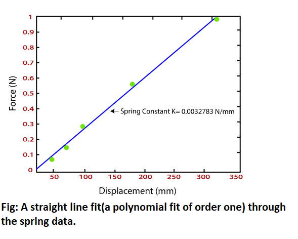 Least squares curve fittingThe procedure of least square curve fit can simply be implemented in MATLAB, because the technique results in a set of linear equations that need to be solved. Most of the curve fits are polynomial curve fits or exponential curve fits (including power laws, e.g., y=axb). Two most commonly used functions are:
1.ln (y)=ln (a) +bx or y =a0+a1 x,where y =ln(y), a1=b,and a0=ln?(a). 2. ln(y)=ln(c) +d ln (x) or y = a0+a1 x, where y = ln (y), a1=d,and a0=ln?(c). Now we can use polyfit in both methods with just first-order polynomials to determine the unknown constants. The steps involved are the following: Step1: Develop new input: Develop new input vectors y and x, as allocate, by taking the log of the original input. For example, to fit the curve of the type y=aebx, create ybar=log(y) and leave x and to fit a curve of the type y=cxd, create ybar=log(y) and xbar=log(x). Step2: Do a linear fit: Use polyfit to found the coefficients a0 and a1for a linear curve fit. Step3: Plot the curve: From the curve fit coefficients, calculates the values of the original constants (e.g., a, b). Recomputed the values of y at the given x's according to the relationship obtained and plot the curve along with the original data. The following are the table shows the time versus pressure variation readings from a vacuum pump. We will fit a curve, P(t)=P0 e-t/τ, through the data, and determine the unknown constants P0 and τ.
By taking the log of both sides of the relationships, we have 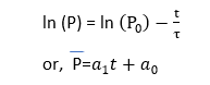 where P=ln(P), a1= Example: Create a script file And plots the following graph: 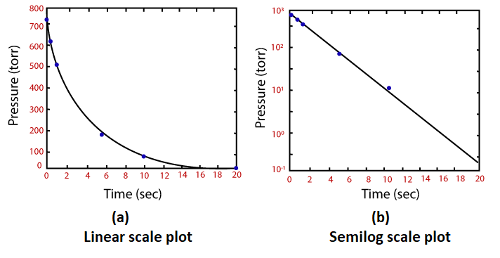
Next TopicMATLAB Interpolation
|
 -and a0=ln?(P0 ). Thus, we can easily computed P0 and τ once we have a1 and a0.